Analyze Amazon order data with Excel

After reading this article, you will be able to carry out detailed evaluations of your financial transactions using existing board tools (e.g. Excel).

We will proceed with this in several steps:

1. Export the data from AMALYTIX
2. Import the data into Excel
3. Evaluation of the data in Excel

Export data from AMALYTIX

In AMALYTIX, you can export almost all data that the tool collects for you as a CSV file. This allows individual analysis that are not shown in the tool. These can be customer-specific questions, for example.

The reports in AMALYTIX can be found under "Reports" (see mark 1 on figure 1).

At first you can set the period you want to analyze. Here we select the data of the last 365 days.

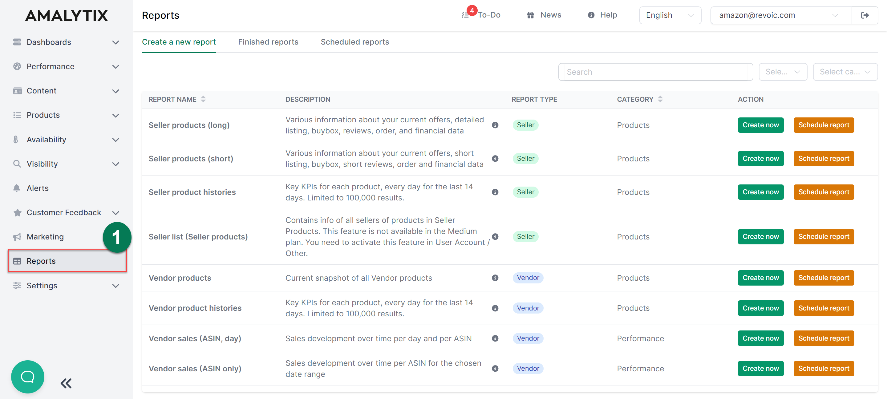
Now select the "Financial" report and then click on "Create".

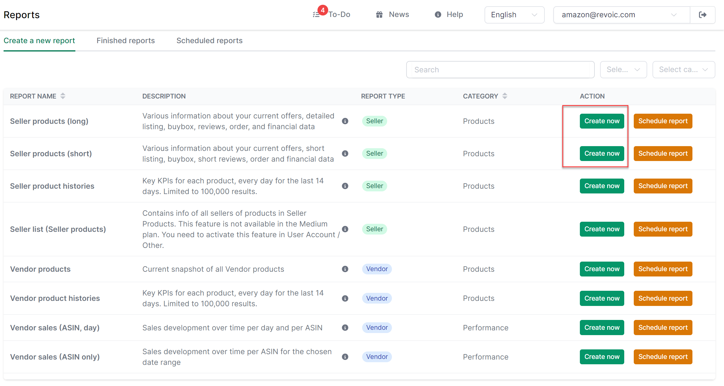
The report is now being generated. You can check the progress of the report generation by clicking the "Refresh list" button.

Once the report has been created, you can download it by clicking on "Download".

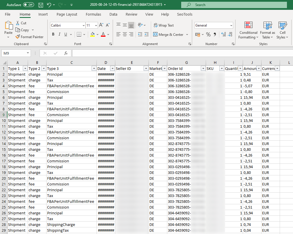
Each individual sales or cost item is listed in this file. The columns indicate the following:

• "Type 1" indicates whether the item is a purchase order ("Shipment"), a return ("Refund") or an item from PPC sales
• "Type 2" indicates whether it is a charge or a fee.
• "Type 3" indicates the exact type. Some of the possible values are as follows:
  • Commission
  • FBAPerUnitFulfillmentFee
  • GiftWrap
  • GiftwrapChargeback
  • GiftWrapTax
  • Goodwill
  • ppcCharges
  • Principal
  • RefundCommission
  • ReturnShipping
  • ShippingCharge
  • ShippingChargeback
  • ShippingHB
  • ShippingTax
  • Tax

The remaining columns are self-explanatory.

The data is intentionally arranged in such a way that it can later be ideally evaluated in pivot tables.

Import the data into Excel

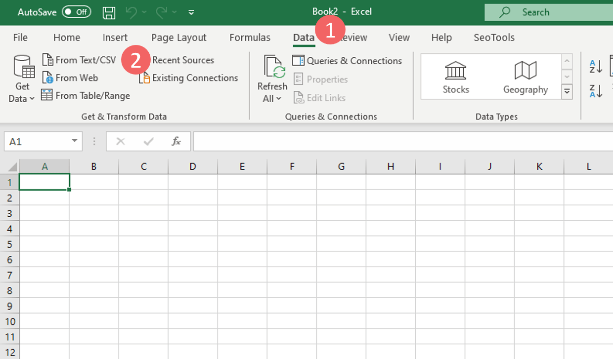
To import the data into Excel, we recommend the import dialog "Data - From text files". To do this, go to the "Data" tab and then click on "From text".

In the following menu, you must select the comma as the separator. Then you can click on "Load", as no further settings are necessary.

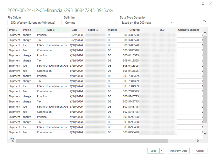
If everything went well, it should now look similar to this in Excel:

Now you can get started with the evaluation.

Evaluation of the data in Excel

To analyze such structured data in Excel, you can use Pivot tables. Pivot tables allow you to group the data in almost any way you like and thus create specific views.

In the following, I would like to introduce you to some of the possibilities. To understand how the pivot table was built, I will illustrate the settings of the pivot tables.

To create an empty pivot table, use the mouse to click somewhere in the table and then go to Insert and there click on "Pivot Table".

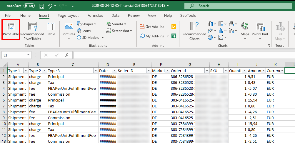
Insert the pivot table as a blank sheet.

Example 1: Sales history for each SKU per month

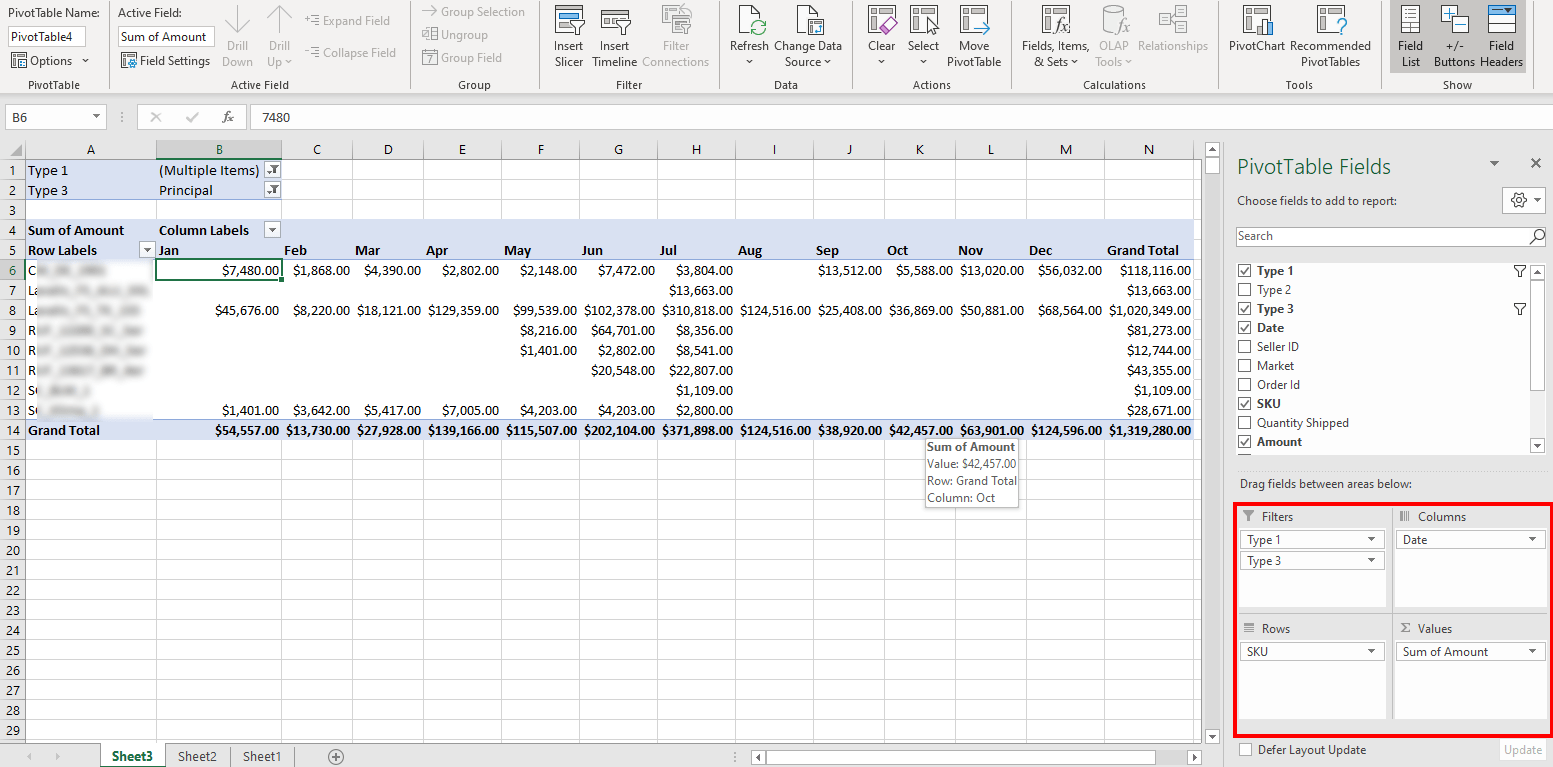
Here the turnover per SKU and month is displayed for the entire period.

The following settings have also been made:

• Filter "Type 1": Only "Revenues" and "Refund" were selected. The revenues are thus reduced by the returns.
• Filter "Type 3": Only "Principal" has been selected to only consider order sales.
• The "Partial results" were deactivated to not receive any intermediate results per year.
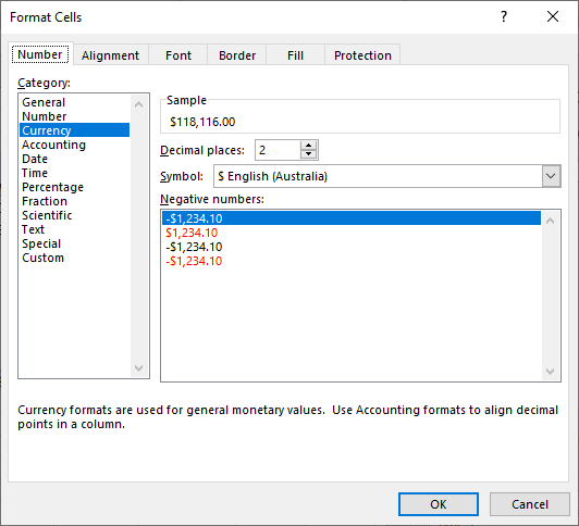
• The number format for "Amount" has been set to "Currency" (see below).
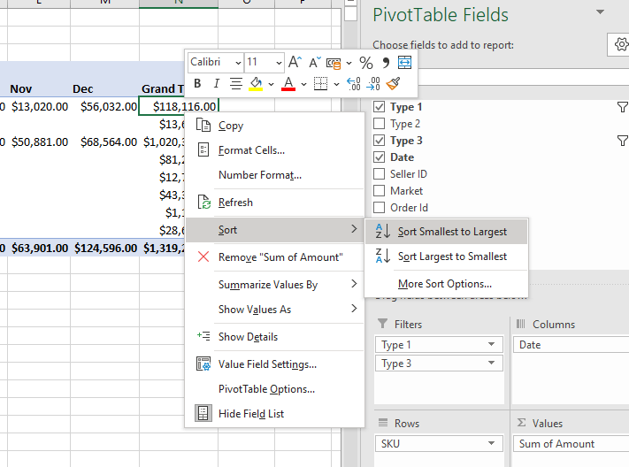
• The rows have been sorted by total sales in descending order so that the SKU with the most sales is at the top.

To sort, right-click on an element in the " Overall Result" column and go to "Sort / Sort by Size (Descending)":

You can change the number format for a value in the "Field settings":

Example 2: Displaying costs in relation to sales

In this example, we show the revenue for 2018 vs. 2019 and compare the costs for vendor fees ("Commission"), for FBA shipping and for PPC costs in relation to the revenue. This is also done with a few clicks without any further action.

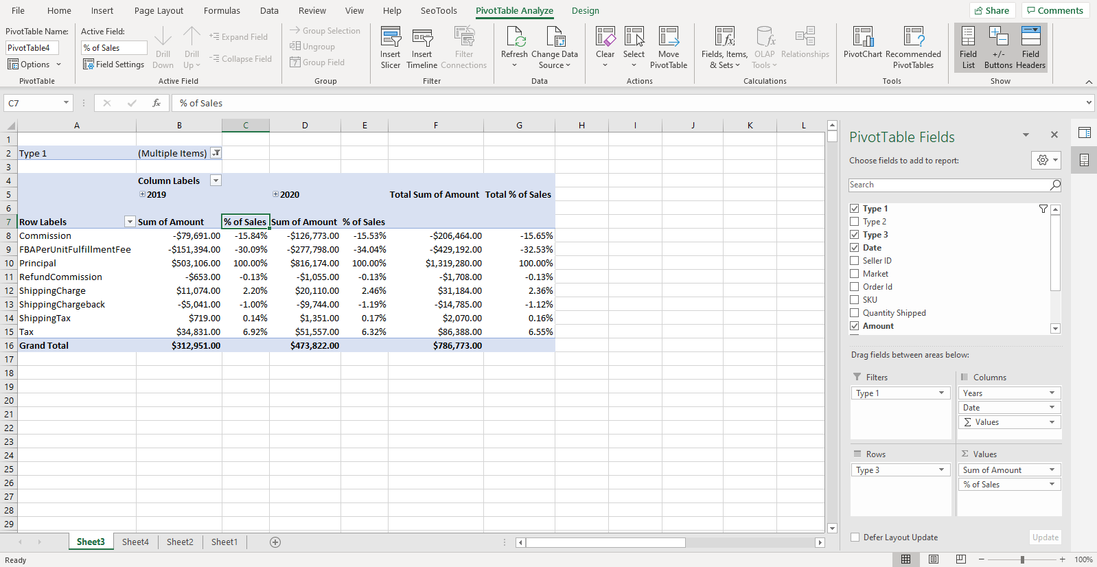
The following parameters are set here:

• Filter "Type 3" on order turnover ("Principal"), PPC costs ("ppcCharges"), vendor fees ("Commission") and FBA shipping fees ("FBAperUnitFulfillmentFee").
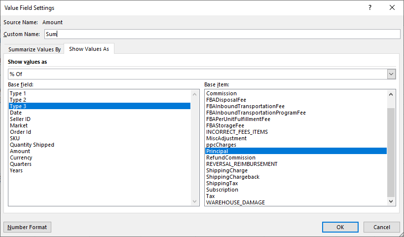
• Under Values, the field "Amount" was created twice. Once normally as a total and once as a percentage of sales (Type 3 / Principal). The latter was created as follows:

Example 3: Working with "Calculated fields"

Within the pivot table, you can also relate columns to each other in any way you like. You can do this using so-called "calculated fields" as the following simple example shows.

In the following we would like to calculate the average sales per product per country.

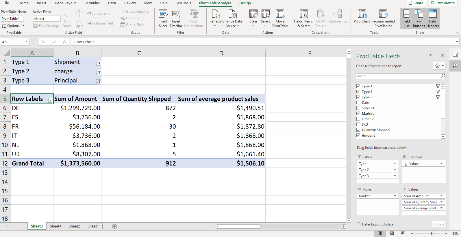
The following settings were defined here:

• Filter "Type 1": Only "Shipments" i.e. orders
• Filter "Type 2": Only "charges" i.e. credit notes
• Filter "Type 3": Only "Principal" i.e. sales

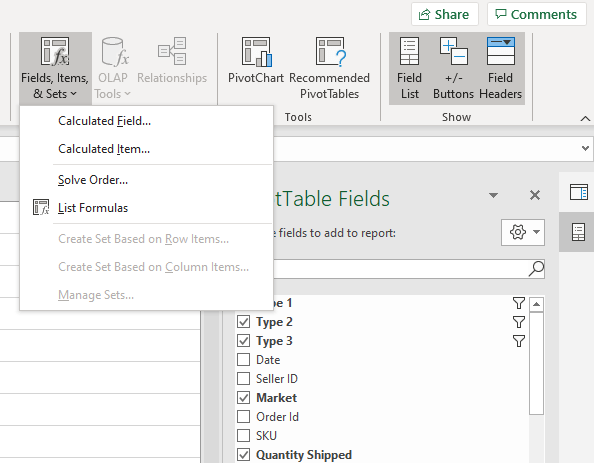
We have inserted the "calculated field" via this menu:

We then defined a field called "Average product sales", where the sales are divided by the number of units ordered.

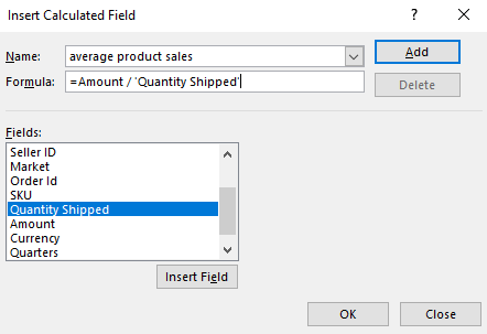
We then added this field to the pivot table.

Conclusion

With the help of the "Payments" report, many more evaluations can be carried out. The examples given are only intended to give you a feeling for what is possible.

Further evaluations become possible if you enrich the "Payments" report with additional reports from AMALYTIX, e.g. with data from the "Product Catalog" report. Here you can then also assign the brand, parent ASIN, category and much more to each SKU and add aggregations on this data.

You have created an interesting report? Send us a (anonymized) screenshot of your analysis. We will be happy to add further practical examples to the article.

In AMALYTIX, we also map standard evaluations such as period comparisons for sellers in our Performance Module. You can compare any periods and key figures.

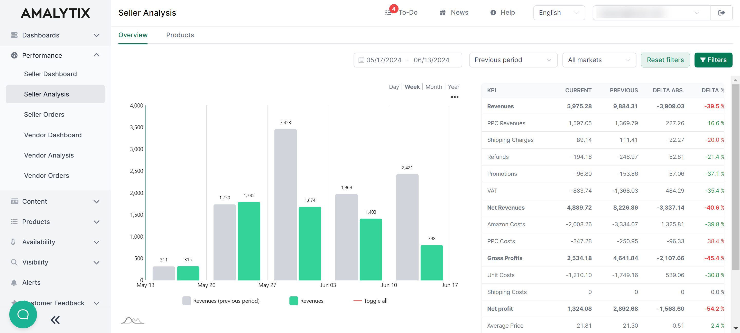
Using the item Aggregation, the values at the level of

• Child ASIN
• Parent ASIN
• Category
• Brand

can be compared.