Analyze the Amazon Brand Analytics search term report with Python and Jupyter Notebooks
Trutz Fries
For brands, Amazon provides the search term report in Brand Analytics to analyze the search and click behavior of Amazon’s customers. This helps to operationalize your Amazon SEO activities.
In this post I want to show you how how to analyze this data using a standard tool like Python, Pandas and Jupyter Notebooks. With some lines of code, we demonstrate how to quickly find the most used search terms, seasonal search terms, a brand’s performance, and much more.
To follow along you need:
- A working installation of Jupyter Lab. We recommend that you install Anaconda.
- Access to Brand Analytics to download the CSV version of the search term report
To make some interesting analyses it makes sense to not only load the current report but e.g. the 52 weeks of reports. You can download those as well in Brand Analytics. Takes some time, but it is doable.
Once you have it, we need to further make some preparations to load and work with it.
Ready? Let’s go!
Setup
First things first. We need to load all necessary libraries:
# Setup
import pandas as pd
import numpy as np
import time

import matplotlib.pyplot as plt
from matplotlib.pyplot import figure
import seaborn as sns
import datetime
from datetime import timedelta
import glob

%config InlineBackend.figure_format='retina'
plt.rcParams["figure.dpi"] = 200
Let’s also define some helper methods. These methods are not necessary if you would like to only analyze the data but we use them here to better show the results in this blog post.
# Get link to an ASIN
def get_ASIN_Link(ASIN, domain="US"):
    if domain == "DE":
      domain = "de"
    elif domain == "US":
      domain = "com"
    link = '<a href="https://www.amazon.' + domain + '/dp/' + ASIN + '" target="_blank">' + ASIN + '</a>'
    return link

# Define a function for colouring (red for negative, changes number format)
def highlight_max(s):
    if s.dtype == np.object:
        is_neg = [False for _ in range(s.shape[0])]
    else:
        is_neg = s < 0
    return ['color: red;' if cell else 'color:black'
        for cell in is_neg]
Define some variables
First, let’s create some variables we can use later on and make changes to our script easier:
# Common
currentWeek  = '33'
previousWeek = '32'
market       = 'US'
yearString   = '2021'

yearWeekCurrent = yearString + '-' + currentWeek
yearWeekPrevious = yearString + '-' + previousWeek

# Variables
pathToProducts = "/your/path/to/products.csv"
columnsInProducts = ['ASIN', 'marketplaceTitle', 'category', 'brand', 'productImageUrl', 'productTitle'] # US, adjust for other markets

pathToReports = "/your/path/to/brandanalyticsdata/"
columnsInReports = ["Search Term","Search Frequency Rank","#1 Clicked ASIN","#2 Clicked ASIN","#3 Clicked ASIN"] # US, adjust for other markets
columnsInReportsSearchTerm = ["Search Term","Search Frequency Rank"] # US, adjust for other markets

thousandSeparator = "," # US, adjust for other markets

# For two weeks based analysis only:
currentWeekPath = pathToReports + "Amazon-Searchterms_US_2021_" + currentWeek + ".csv"
previousWeekPath = pathToReports + "Amazon-Searchterms_US_2021_" + previousWeek + ".csv"
Our script expects that your files should follow the following naming format:
...
Amazon-Searchterms_US_2021_27.csv
Amazon-Searchterms_US_2021_28.csv
Amazon-Searchterms_US_2021_29.csv
Amazon-Searchterms_US_2021_30.csv
Amazon-Searchterms_US_2021_31.csv
Amazon-Searchterms_US_2021_32.csv
Amazon-Searchterms_US_2021_33.csv
...
This allows us later to extract the marketplace, the year, and the calendar week from the filename. This data will be added later to our data frame to allow for time series analysis.
Here is a quick tip: As Amazon’s search term reports are quite large (1 Mio. lines per week) you can shorten those via this quick shell script you can run e.g. in a bash shell:
for file in ./csv/Amazon*.csv; do
    head -n 500000 "$file" > "short/$file"
done
This will reduce each file to the first 500,000 lines and save a short version to the short folder. If you analyze e.g. 1 year of data this will reduce the speed of your analyses significantly.
Importing Brand Analytics search term data
First, we need to load all search term reports into memory. Again, the script expects that these files sit together in a single directory with some strict naming conditions:
# Initialze empty dataframe we'll append data to
dfFinal = pd.DataFrame()
# Get all files
all_files = sorted(glob.glob(pathToReports + "/*.csv"))
print ('\n'.join(all_files))
# Import files to df
i = 0
for file in all_files:
i = i + 1
print(str(i) + ". " + file)
# Read from CSV file
dfTemp = pd.read_csv(file, thousands=thousandSeparator, usecols=columnsInReports, engine="python", error_bad_lines=True, encoding='utf-8', skiprows=1, sep=",")
# Add week from filename to dataframe as new column
week = file[-6:][:2] # e.g. 06
year = file[-11:][:4] # e.g. 2020
yearWeek = year + '-' + week # e.g. 2020-06
marketplaceTitle = file[-14:][:2]
dfTemp['week'] = week
dfTemp['year'] = year
dfTemp['yearWeek'] = yearWeek
dfTemp['marketplaceTitle'] = marketplaceTitle
# Concat with previous results
dfFinal = pd.concat([dfTemp, dfFinal])
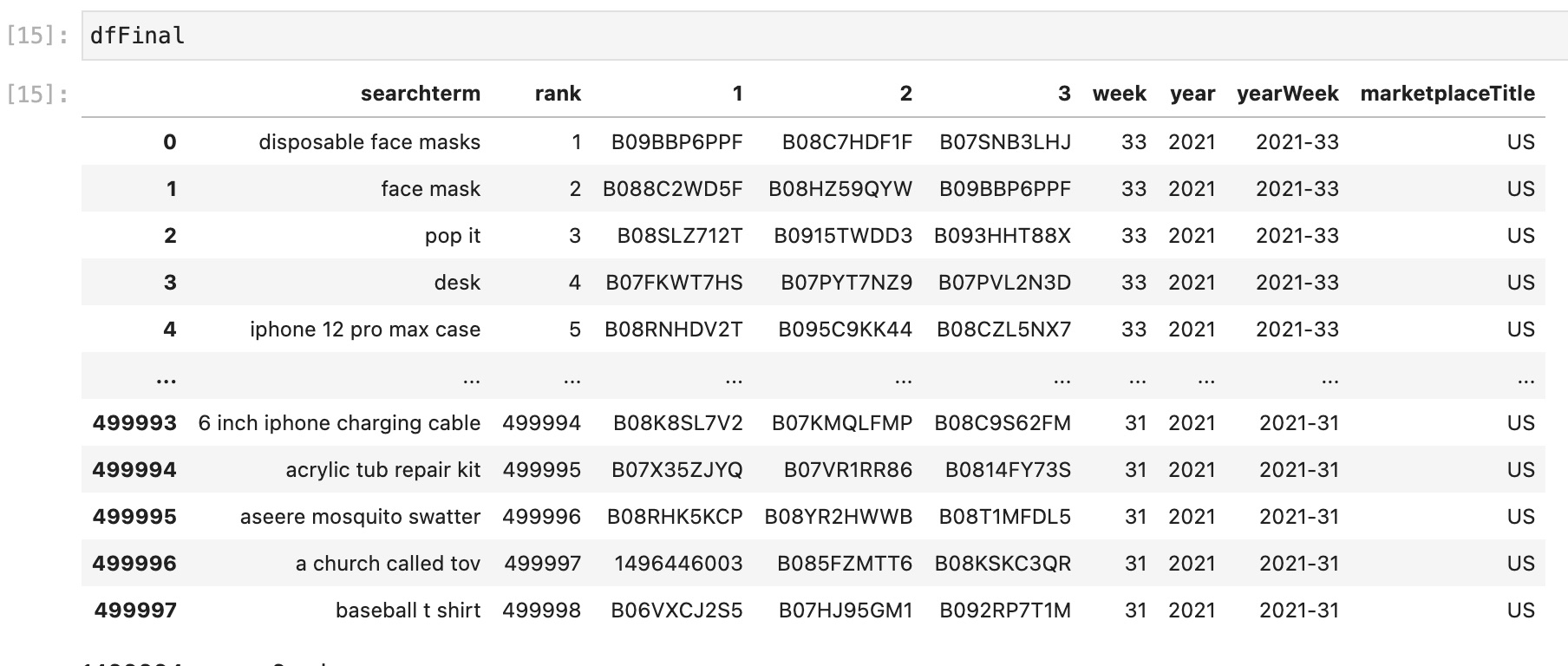
# We rename ASIN1 into `1` as this becomes handy when we unmelt the report
dfFinal.columns = ['searchterm', 'rank', '1', '2', '3', 'week', 'year', 'yearWeek', 'marketplaceTitle']
# Change data type to int
dfFinal = dfFinal.astype({"week": int, "year": int, "year": int})
Some of the analyses shown below only require loading the current and the previous week of data. If you want to do that, you can just load the 2 respective files, e.g. like this:
dfCurrent = pd.read_csv(currentWeekPath, thousands=thousandSeparator, usecols=columnsInReportsSearchTerm, engine="python", error_bad_lines=True, encoding='utf-8', skiprows=1,  sep=",")

dfPrevious= pd.read_csv(previousWeekPath, thousands=thousandSeparator, usecols=columnsInReportsSearchTerm, engine="python", error_bad_lines=True, encoding='utf-8', skiprows=1,  sep=",")
The thousandSeparator parameter depends on your locale. It’s either the dot or a comma. For US reports it is the comma.
We will need to unmelt all this data. More on that soon.
Before we also load some products data (e.g. the brand) for each ASIN found in all search term report files which will be handy to enrich the data later:
dfProducts = pd.read_csv(pathToProducts, engine="python", error_bad_lines=True, encoding='utf-8', sep=",")
If you don’t have this data, you can extract this with some work from the product title of the search term reports. However, this is not covered here.
Re-formatting / shaping the data
Next, we need to bring our data into the right format. Basically, we need to “unpivot” the data we have which will make the following analyses possible.
Pandas provides a very handy function for that called melt (see documentation), which makes this very easy:
# Unmelt dataframe

# Create a copy
dfWideMultiReports = dfFinal

# Unmelt from wide to long
dfWideMultiReportsLong = dfWideMultiReports.melt(id_vars=["searchterm", "rank", "week", "year", "yearWeek", "marketplaceTitle"], var_name="position", value_name="ASIN")

# Add column with a 1 so we can sum by this colum
dfWideMultiReportsLong['count'] = 1

# Make position an int
dfWideMultiReportsLong = dfWideMultiReportsLong.astype({"position": int})
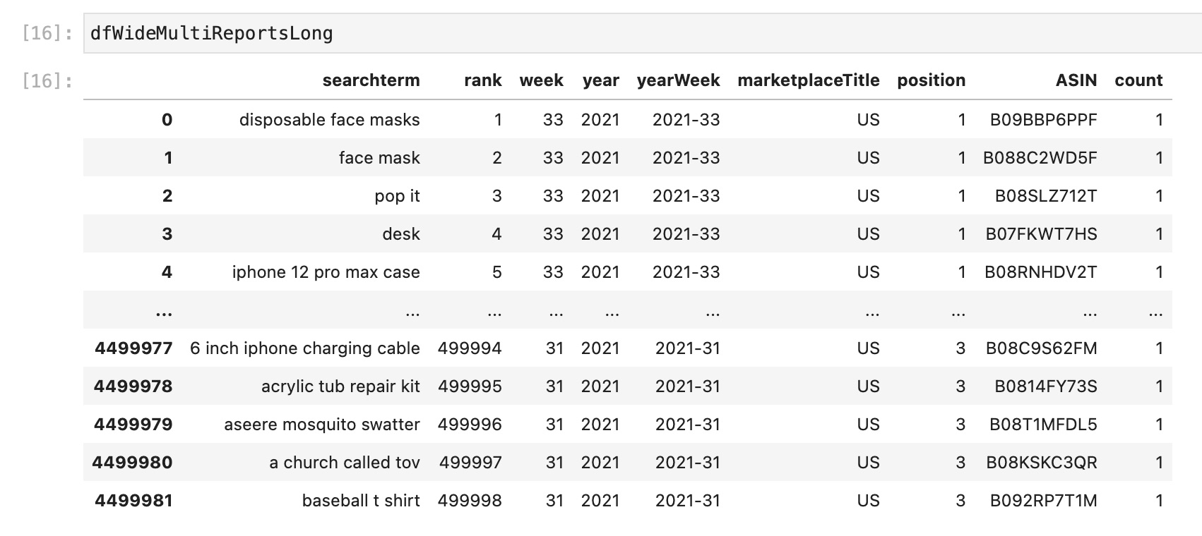
Now we have one row for each search term, ASIN, week combination.
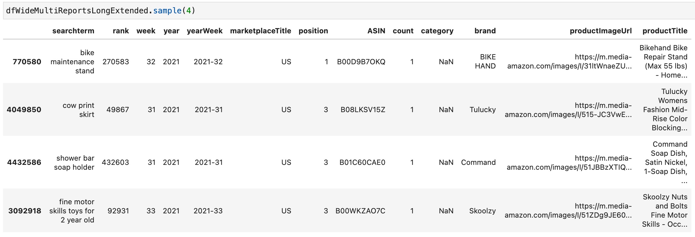
Next, we enrich our search term report data with the product data to e.g. have a column for the ASIN’s brand:
# Left join products data to searchterm data
dfWideMultiReportsLongExtended = pd.merge(left=dfWideMultiReportsLong, right=dfProducts, how='left', left_on=['marketplaceTitle','ASIN'], right_on = ['marketplaceTitle','ASIN'])

# Drop rows where searchterm or brand is NaN
dfWideMultiReportsLongExtended = dfWideMultiReportsLongExtended.dropna(subset=['searchterm', 'ASIN', 'rank', 'week', 'year', 'yearWeek', 'marketplaceTitle', 'position', 'brand', 'productTitle']) # Only dop rows with N/A in specific columns
We also drop rows where we are missing some data using the dropna method.
The final dataframe we are going to work with looks like this now:
Analysis of the data
Now as we have everything in place we can start doing some simple analysis. We will start by analyzing changes between the current and the previous week. As shown above we have this data in our dfCurrent and dfPrevious dataframes.
We will look at:
- Search terms
- Brands
- Products
Search term analysis
Prepare the data
We need to merge our 2 dataframes containing the current and the previous week of data for some analyses.
# Change column names
dfCurrent.columns = ['searchterm', 'currentRank']
dfPrevious.columns = ['searchterm', 'previousRank']

# Make currentRank and previousRank an integer
dfCurrent = dfCurrent.astype({"currentRank": int})
dfPrevious = dfPrevious.astype({"previousRank": int})

# Merge current and previous dataframes
dfMerged = pd.merge(left=dfCurrent, right=dfPrevious, how='left', left_on=['searchterm'], right_on = ['searchterm'])
dfPrevious = dfPrevious.astype({"previousRank": int})

# Calculate the changes between current and previous
dfMerged['DeltaAbs']=dfMerged['currentRank']-dfMerged['previousRank']

# Positive value of Change (to see biggest movers in absolute terms)
dfMerged['DeltaAbsPos']=dfMerged['DeltaAbs'].abs()
With that out of the way, let’s do some more fun stuff.
Get the top search terms of the current week
Let’s start slow with some simple tables. Let’s get the top search terms from the current week and show the difference to the previous week. We also add some colors based on the changes using TailwindCSS classes. However, this is not necessary for the sole analysis of the data. It just makes the following tables prettier.
# Get current Top 10 with previous
dfTop10Searchterms = dfMerged
dfTop10Searchterms = dfTop10Searchterms.drop('DeltaAbsPos', 1)

dfTop10Searchterms.columns = ['Searchterm', 'Rank cur.', 'Rank prev.', 'Change']
dfTop10Searchterms['Change'] = dfTop10Searchterms.apply(lambda row: '<span class="text-green-600">↑ ' + str(int(np.nan_to_num(row.Change))) + '</span>' if row.Change < 0 else '<span class="text-red-600">↓ ' + str(int(np.nan_to_num(row.Change))) + '</span>', axis=1)
searchTermsTop = dfTop10Searchterms.head(10).to_markdown(index=False)
The dfTop10Searchterms dataframe looks like this then:
| Searchterm | Rank cur. | Rank previous | Change |
|---|---|---|---|
| disposable face masks | 1 | 1 | ↓ 0 |
| face mask | 2 | 2 | ↓ 0 |
| pop it | 3 | 3 | ↓ 0 |
| desk | 4 | 5 | ↑ -1 |
| iphone 12 pro max case | 5 | 7 | ↑ -2 |
| earbuds | 6 | 6 | ↓ 0 |
| n95 mask | 7 | 4 | ↓ 3 |
| apple watch band | 8 | 11 | ↑ -3 |
| black disposable face masks | 9 | 24 | ↑ -15 |
| laptop | 10 | 15 | ↑ -5 |
The search term black disposable face masks has quite improved compared to the previous week. Remember, the lower the search frequency rank, the more often this term is searched on Amazon.
Get newcomer search terms
Now we can try to find the top search terms (based on search frequency rank) where there was no search frequency rank in the previous week:
# Get new entries where there was no rank in previous week
dfTopNewcomer = dfMerged[dfMerged['previousRank'].isnull()]
dfTopNewcomer = dfTopNewcomer.drop(['previousRank','DeltaAbs', 'DeltaAbsPos'], 1)
dfTopNewcomer = dfTopNewcomer.sort_values(by=['currentRank'], ascending=True).head(10)

dfTopNewcomer.columns = ['New searchterms', 'Rank cur.']
searchTermsNewcomer=dfTopNewcomer.head(10).to_markdown(index=False)
This will e.g. look like this:
| New searchterms | Rank cur. |
|---|---|
| pixel 5a 5g case | 2027 |
| infinity game table | 2459 |
| cicy bell womens casual blazer | 5234 |
| donsfield lint remover | 6945 |
| go oats oatmeal in a ball | 9887 |
| ivernectin | 10034 |
| go oats | 10367 |
| ruthless empire rina kent | 10711 |
| cicy bell blazer | 11057 |
| pixel 5a 5g screen protector | 11222 |
As you can see these are very often long-tail keywords.
Find search terms with the highest rank change
Now let’s look at the “mover’s and shakers” of high-traffic search terms. With “high-traffic” we mean that we reduce the result to search terms with a search frequency rank below 1,000. Feel free to play with this parameter to get different results.
# Only include searchterms which are now < 1000
filterWinners = (dfMerged['currentRank'] < 1000)

# Winners
dfWinners = dfMerged[filterWinners].sort_values(by=['DeltaAbs'], ascending=True).head(10)

# Drop DeltaAbsPos column
dfWinners = dfWinners.drop('DeltaAbsPos', 1)

# Rename columns
dfWinners.columns = ['Searchterm', 'Rank CW ' + currentWeek, 'Rank CW ' + previousWeek, 'Delta']
For the winners this will look like this:
| Searchterm | Rank CW 33 | Rank CW 32 | Delta |
|---|---|---|---|
| black american flags | 847 | 14,708 | -13,861 |
| paw patrol movie | 523 | 4,817 | -4,294 |
| sexy dresses for women | 762 | 2,924 | -2,162 |
| headphones for kids for school | 869 | 2,460 | -1,591 |
| room decor aesthetic | 825 | 2,373 | -1,548 |
| hunger games | 996 | 2,412 | -1,416 |
| eyebrow pencil | 480 | 1,859 | -1,379 |
| throw pillow covers | 355 | 1,641 | -1,286 |
| bentgo kids lunch box | 705 | 1,902 | -1,197 |
| respect | 927 | 2,076 | -1,149 |
Top movers
Let’s find out for which high-traffic search terms (again with a search frequency rank below 1,000) the search frequency rank has changed most compared to the previous week. We include both positive and negative changes as we sort by the absolute changes here.
# Top Movers within a certain rank threshold
filterMovers = (dfMerged['previousRank'] < 1000) & (dfMerged['currentRank'] < 1000)
dfMerged = dfMerged.astype({"currentRank": float}) # Needs to be there otherwise currentRank column is string?!
dfMovers = dfMerged[filterMovers].sort_values(by=['DeltaAbsPos'], ascending=False).head(10)
dfMovers['DeltaAbs'] = dfMovers.apply(lambda row: '<span class="text-green-600">↑ ' + str(int(np.nan_to_num(row.DeltaAbs))) + '</span>' if row.DeltaAbs < 0 else '<span class="text-red-600">↓ ' + str(int(np.nan_to_num(row.DeltaAbs))) + '</span>', axis=1)

# Drop DeltaAbs column
dfMovers = dfMovers.drop('DeltaAbsPos', 1)

# Rename columns
dfMovers.columns = ['Searchterm', 'Rank CW ' + currentWeek, 'Rank CW ' + previousWeek, 'Delta']
The result looks like this:
| Searchterm | Rank CW 33 | Rank CW 32 | Delta |
|---|---|---|---|
| field of dreams | 998 | 196 | ↓ 802 |
| friday the 13th | 902 | 210 | ↓ 692 |
| pop it fidget toys | 241 | 929 | ↑ -688 |
| n95 masks for virus protection | 911 | 395 | ↓ 516 |
| wireless earbuds bluetooth | 302 | 785 | ↑ -483 |
| college essentials | 875 | 454 | ↓ 421 |
| fall clothes for women | 297 | 678 | ↑ -381 |
| air conditioner | 583 | 206 | ↓ 377 |
| usb c cable | 618 | 991 | ↑ -373 |
| iphone charging cords | 949 | 594 | ↓ 355 |
Of course, you can change the thresholds as you like.
Brand analyses
If we have the brand attached to each entry, we can also analyze by brand. Here we use our big data frame instead of the 2 separate weeks.
Let’s find out which brands show up most often:
filtCurrentWeek = (dfWideMultiReportsLongExtended['yearWeek'] == yearWeekCurrent)
filtPreviousWeek = (dfWideMultiReportsLongExtended['yearWeek'] == yearWeekPrevious)

dfBrandCurrentWeek = dfWideMultiReportsLongExtended[filtCurrentWeek]
dfBrandPreviousWeek = dfWideMultiReportsLongExtended[filtPreviousWeek]

dfTopBrandsCurrentWeek = dfBrandCurrentWeek['brand'].value_counts().sort_values(ascending=False).to_frame('countCurrent')
dfTopBrandsPreviousWeek = dfBrandPreviousWeek['brand'].value_counts().sort_values(ascending=False).to_frame('countPrevious')

brandsTop = dfTopBrandsCurrentWeek.head(10).to_markdown().replace('countCurrent', 'Count')
The brandsTop dataframe will look like this:
| Count | |
|---|---|
| Amazon Basics | 9670 |
| Apple | 5620 |
| Nike | 5469 |
| 365 by Whole Foods Market | 3577 |
| adidas | 3546 |
| SAMSUNG | 3171 |
| Amazon | 3079 |
| HP | 3002 |
| Generic | 2809 |
| LEGO | 2737 |
We just count by a brand’s appearance in the search term report. You could include the search frequency rank to give search terms with a low rank a higher weight. This was not done here.
Let’s now find out which brands have improved compared to the previous week. Again we do a plain count here:
dfTopBrandsMerged = dfTopBrandsCurrentWeek.merge(dfTopBrandsPreviousWeek, how='left', left_index=True, right_index=True)
dfTopBrandsMerged['DeltaAbs'] = dfTopBrandsMerged['countCurrent'] - dfTopBrandsMerged['countPrevious']
dfTopBrandsMerged['DeltaAbsPos'] = dfTopBrandsMerged['DeltaAbs'].abs()

# Winners and Losers
dfBrandLoosers = dfTopBrandsMerged.sort_values(by=['DeltaAbs'], ascending=True).head(10)

dfBrandWinners = dfTopBrandsMerged.sort_values(by=['DeltaAbs'], ascending=False).head(10)
dfBrandWinners.columns = ['# CW ' + currentWeek, '# CW ' + previousWeek, 'Delta', 'Delta Abs']
dfBrandWinners = dfBrandWinners.drop('Delta Abs', 1)
brandsWinner = dfBrandWinners.to_markdown()
The brandsWinner dataframe will look like this:
| # CW 33 | # CW 32 | Delta | |
|---|---|---|---|
| Amazon | 3079 | 2833 | 246 |
| SAMSUNG | 3171 | 2939 | 232 |
| Bentgo | 814 | 638 | 176 |
| HP | 3002 | 2863 | 139 |
| Disguise | 820 | 690 | 130 |
| Texas Instruments | 718 | 589 | 129 |
| DXLOVER | 249 | 131 | 118 |
| Generic | 2809 | 2696 | 113 |
| Logitech | 1208 | 1095 | 113 |
| Spooktacular Creations | 293 | 182 | 111 |
Product analyses
What we did with search terms and brands can also be done with products. Let’s look for the products which show up most or more often compared to the previous week. We will use our full data set again here.
First, we’ll filter the big dataset, then we’ll merge the current and the previous week, and then we’ll count the number of occurrences.
filtCurrentWeek = (dfWideMultiReportsLongExtended['yearWeek'] == yearWeekCurrent)
filtPreviousWeek = (dfWideMultiReportsLongExtended['yearWeek'] == yearWeekPrevious)

dfProductCurrentWeek = dfWideMultiReportsLongExtended[filtCurrentWeek]
dfProductPreviousWeek = dfWideMultiReportsLongExtended[filtPreviousWeek]

dfTopProductsCurrentWeek = dfProductCurrentWeek['ASIN'].value_counts().sort_values(ascending=False).to_frame('countCurrent')
dfTopProductsPreviousWeek = dfProductPreviousWeek['ASIN'].value_counts().sort_values(ascending=False).to_frame('countPrevious')

# ASIN is index, create column from it, add marketplaceTitle for making the merge possible
dfTopProductsCurrentWeek['ASIN'] = dfTopProductsCurrentWeek.index
dfTopProductsCurrentWeek['marketplaceTitle'] = market

dfTopProductsPreviousWeek['ASIN'] = dfTopProductsPreviousWeek.index
dfTopProductsPreviousWeek['marketplaceTitle'] = market

# Add product data, e.g. product title
dfTopProductsCurrentWeek = pd.merge(left=dfTopProductsCurrentWeek, right=dfProducts, how='left', left_on = ['marketplaceTitle', 'ASIN'], right_on = ['marketplaceTitle', 'ASIN'])

# Merge current with previous df
dfTopProductsMerged = dfTopProductsCurrentWeek.merge(dfTopProductsPreviousWeek, how='left', left_on = ['marketplaceTitle', 'ASIN'], right_on = ['marketplaceTitle', 'ASIN'])

# Calculate the changes
dfTopProductsMerged['DeltaAbs'] = dfTopProductsMerged['countCurrent'] - dfTopProductsMerged['countPrevious']
dfTopProductsMerged['DeltaAbsPos'] = dfTopProductsMerged['DeltaAbs'].abs()

# Shorten the product title and add ASIN
dfTopProductsMerged['productTitleShort'] = dfTopProductsMerged['productTitle'].astype(str).replace('|', '-').str[0:30] + ' (' + get_ASIN_Link(dfTopProductsMerged['ASIN']) + ')'

# Get rid of some columns and prepare output
dfTopProductsForOutput = dfTopProductsMerged[['productTitleShort', 'countCurrent']]
dfTopProductsForOutput.columns = ['Product title', 'Count']

productsTop = dfTopProductsForOutput.head(10).to_markdown(index = False)

# Winners
dfProductsWinners = dfTopProductsMerged.sort_values(by=['DeltaAbs'], ascending = False)
dfProductsWinners = dfProductsWinners[['productTitleShort', 'DeltaAbs' ]]
dfProductsWinners.columns = ['Product title', 'Delta']
productsWinner = dfProductsWinners.head(10).to_markdown(index=False)

# Loosers
dfProductsLoosers = dfTopProductsMerged.sort_values(by=['DeltaAbs'], ascending = True)
dfProductsLoosers = dfProductsLoosers[['productTitleShort', 'DeltaAbs' ]]
dfProductsLoosers.columns = ['Product title', 'Delta']
productsLoser = dfProductsLoosers.head(10).to_markdown(index=False)
The first rows of productsTop look like this then:
| Product title | Count |
|---|---|
| EnerPlex 3-Ply Reusable Face M (B088C2WD5F) | 287 |
| Matein Travel Laptop Backpack, (B06XZTZ7GB) | 226 |
| Blink Mini – Compact indoor pl (B07X6C9RMF) | 219 |
| Gildan Men’s Crew T-Shirts, Mu (B091FNSFN1) | 210 |
| Crocs Men’s and Women’s Classi (B09BBT7T3P) | 207 |
| AIHOU 50PC Kids Butterfly Disp (B08LL8H78D) | 195 |
| Apple AirPods Pro (B07ZPC9QD4) | 195 |
| Beckham Hotel Collection Bed P (B01LYNW421) | 179 |
| Apple AirPods with Charging Ca (B07PXGQC1Q) | 177 |
| TCP Global Salon World Safety (B08FXLVHTY) | 176 |
Again we only count the appearance. We have not weighted this by the search frequency rank of the respective keywords.
Respectively productsWinner looks like this:
| Product title | Delta |
|---|---|
| KATCHY Indoor Insect and Flyin (B07B6RZP4H) | 160 |
| Texas Instruments TI-84 Plus C (B00TFYYWQA) | 64 |
| 5 Layer Protection Breathable (B08F8Y3X59) | 59 |
| Columbia Baby Girls’ Benton Sp (B077FNDN8N) | 55 |
| Fire 7 Kids Edition Tablet, 7” (B07H936BZT) | 54 |
| BISSELL Crosswave All in One W (B01DTYAZO4) | 51 |
| $20 PlayStation Store Gift Car (B004RMK4BC) | 50 |
| Germ Guardian True HEPA Filter (B004VGIGVY) | 50 |
| Texas Instruments TI-84 PLUS C (B00XOLOOPY) | 47 |
| SPACE JAM Heroes of Goo JIT Zu (B08S3GWM5W) | 44 |
Let’s now find out which are the hottest newcomer products and which products showed high changes. The code looks for this looks like this:
# Best newcoming products
filtBothWeeks = (dfWideMultiReportsLongExtended['yearWeek'] == yearWeekCurrent) | (dfWideMultiReportsLongExtended['yearWeek'] == yearWeekPrevious)
dfProductCurrentWeek = dfWideMultiReportsLongExtended[filtBothWeeks]

df_pivot_current = pd.pivot_table(dfProductCurrentWeek,index=["ASIN"], columns=["yearWeek"], values=["searchterm", "rank"],aggfunc={"searchterm":len,"rank":min})
df_pivot_current['marketplaceTitle'] = market
df_pivot_current.columns= ['minRankPrevious', 'minRankCurrent', 'countPrevious', 'countCurrent', 'marketplaceTitle']
df_pivot_current.reset_index(inplace = True)

df_pivot_current.sort_values(by=['countCurrent'], ascending = False)

df_pivot_current['countDelta'] = df_pivot_current['countCurrent'] - df_pivot_current['countPrevious']
df_pivot_current.sort_values(by=['countDelta'], ascending = False)

# Add product data, e.g. product title
df_pivot_current_ext = pd.merge(left=df_pivot_current, right=dfProducts, how='left', left_on = ['marketplaceTitle', 'ASIN'], right_on = ['marketplaceTitle', 'ASIN'])

# Shorten the product title and add ASIN
df_pivot_current_ext['productTitleShort'] = df_pivot_current_ext['productTitle'].astype(str).replace('|', '-').str[0:30] + ' (' + get_ASIN_Link(df_pivot_current_ext['ASIN'], market) + ')'

# Products with most change between current an prev. week
df_pivot_current_ext_short = df_pivot_current_ext[['productTitleShort', 'countCurrent', 'minRankCurrent', 'countDelta']]
df_pivot_current_ext_short = df_pivot_current_ext_short.sort_values(by=['countDelta'], ascending = False)
df_pivot_current_ext_short.columns = ['Product title', '# searchterms', 'Best rank', 'Delta']

productsNewcomer = dfTopProductNewcomer.head(10).to_markdown(index=False)
Let’s look at the movers and shakers first:
| Product title | # searchterms | Best rank | Delta |
|---|---|---|---|
| KATCHY Indoor Insect and Flyin (B07B6RZP4H) | 174 | 775 | 160 |
| Texas Instruments TI-84 Plus C (B00TFYYWQA) | 82 | 1914 | 64 |
| 5 Layer Protection Breathable (B08F8Y3X59) | 92 | 1276 | 59 |
| Columbia Baby Girls’ Benton Sp (B077FNDN8N) | 58 | 2817 | 55 |
| Fire 7 Kids Edition Tablet, 7” (B07H936BZT) | 66 | 1387 | 54 |
| BISSELL Crosswave All in One W (B01DTYAZO4) | 91 | 5223 | 51 |
| Germ Guardian True HEPA Filter (B004VGIGVY) | 98 | 149 | 50 |
| $20 PlayStation Store Gift Car (B004RMK4BC) | 66 | 6829 | 50 |
| Texas Instruments TI-84 PLUS C (B00XOLOOPY) | 65 | 1914 | 47 |
| SPACE JAM Heroes of Goo JIT Zu (B08S3GWM5W) | 52 | 1277 | 44 |
Let’s figure out which are the best newcomer products:
# Best Newcomer Products (without rankings in previous week)
dfTopProductNewcomer = df_pivot_current_ext[df_pivot_current_ext['countPrevious'].isnull()]
dfTopProductNewcomer = dfTopProductNewcomer.sort_values(by=['countCurrent'], ascending = False)
dfTopProductNewcomer['productTitleShort'] = dfTopProductNewcomer['productTitle'].astype(str).replace('|', '-').str[0:30] + ' (' + get_ASIN_Link(dfTopProductNewcomer['ASIN'], market) + ')'

dfTopProductNewcomer = dfTopProductNewcomer[['productTitleShort', 'countCurrent', 'minRankCurrent']]
dfTopProductNewcomer = dfTopProductNewcomer.sort_values(by=['countCurrent'], ascending = False)
dfTopProductNewcomer.columns = ['Product title', '# searchterms', 'Best rank']
productsNewcomer looks like this:
| Product title | # searchterms | Best rank |
|---|---|---|
| adidas Unisex-Child Questar Fl (B08TK7P6CN) | 160 | 1966 |
| Kids KN95 Face Mask - 25 Pack (B08Q8J5MNQ) | 142 | 844 |
| Crocs Unisex-Child Kids’ Class (B08LDBPB3J) | 50 | 2595 |
| TeeTurtle - The Original Rever (B088X4XFNQ) | 47 | 10620 |
| adidas Women’s Grand Court Sne (B09746H9SC) | 45 | 588 |
| Kids Face Mask, Disposable Kid (B08R8CHZN3) | 40 | 17142 |
| Potaroma Cat Wall Toys, 7.7 by (B08T9CL5T9) | 31 | 16802 |
| MIAODAM Face Mask Lanyards, Ma (B09CDDP2Z3) | 28 | 279 |
| KN95 Particulate Respirator - (B0876J4F4Y) | 27 | 235 |
| Earbuds Earphones Wired Stereo (B098L2DSS3) | 26 | 3532 |
Additional Amazon Keyword and Brand Analyses
We can do so much more with this data. Let me show you some examples:
Single keyword analysis by week
Once we have loaded the data for e.g. the last 52 weeks we can plot the development of a single search term over time:
searchTerm = "pool"

# Filter data
dfSingleKeyword = dfFinal.loc[dfFinal['searchterm'] == searchTerm].sort_values('week')

# Plot the data
kwPlot = dfSingleKeyword.plot(x ='week', y='rank', figsize=(10,6), title="Keyword: " + searchTerm)
kwPlot.set_xlabel("Weeks")
kwPlot.set_ylabel("Rank")
kwPlot
This will give us a better understanding of how the demand for certain products behaves over time.
Here is a graph for the term “pool” shown above.
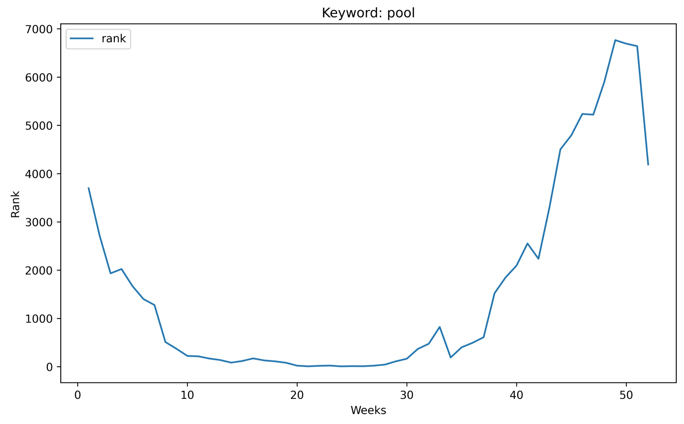
It’s easy to see when the pool season started and ended in 2021.
Show generic search terms a specific brand ranks for
Here we search for all search terms the brand “OPPO” ranks for but does not include the brand’s name. Sorted by rank ascending.
Here we assume that the data for a single brand analytics report sits in the dataframe called df:
# Show searchterms for a given brand and sort by rank ASC
myFilter = (df['brand'] == 'OPPO') & (df["Searchterm"].str.contains('oppo')==False)
df.loc[myFilter].sort_values(by=['Rank'])
This should give us generic search terms.
This of course can also be done for multiple brands across multiple reports:
brands = ["Kasa Smart", "ARENTI", "GW Security", "Blink Home Security"]
brandsLowerCase = [x.lower() for x in brands]
# Get all rows from selected brands
dfBrandTerms = dfWideMultiReportsLongExtended[dfWideMultiReportsLongExtended.brand.isin(brands)]
# Group result
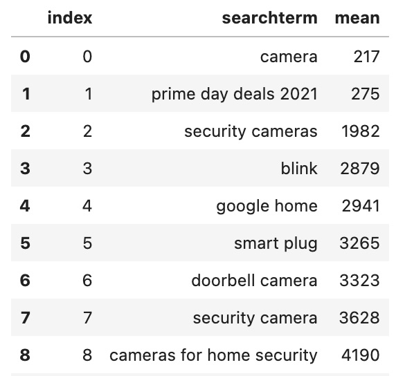
dfBrandTermsGrouped = dfBrandTerms.groupby('searchterm')['rank'].agg(['mean']).sort_values(by=['mean'])
# Reset index
dfBrandTermsGrouped.reset_index(level=0, inplace=True)
dfBrandTermsGrouped = dfBrandTermsGrouped.astype({"mean": int})
The dfBrandTermsGrouped dataframe now looks like this:
If we only want to find generic keywords, let’s remove the search terms which include a brand’s name:
brandKeywordsWithoutBrand = dfBrandTermsGrouped[~dfBrandTermsGrouped.searchterm.str.contains('|'.join(brandsLowerCase))]
Want to export both all and non-brand keywords to Excel? Pandas has you covered:
with pd.ExcelWriter('camera-export-brand-keywords.xlsx') as writer:
    brandKeywordsWithoutBrand.to_excel(writer, sheet_name='Generic Keywords', float_format="%.2f")
    dfBrandTermsGrouped.to_excel(writer, sheet_name='All Keywords', float_format="%.2f")
Classify search terms
We could even go one step further and try to classify this for every search term in the report using this function.
To do this, we first need to put all brands into a list:
# Get unique list of brands
dfWideMultiReportsLongExtended['brand'].nunique()
allBrands = dfWideMultiReportsLongExtended.brand.unique()

# Lower each name
allBrands = [ x.lower() for x in allBrands if len(str(x)) > 3 ]
Now we can analyze each row in our dataframe and check if the search term contains the brand’s brand name, the brand name of a different brand, or is a generic searchterm.
def searchTermType (row):
    brand = str(row['brand']).lower()
    searchterm = str(row['searchterm']).lower()

    if (not pd.isnull(brand)) & (brand in searchterm):
        return 'brand'
    if not pd.isnull(brand):
        for brand2 in allBrands:
            if not pd.isnull(brand2):
                if brand2.lower() in searchterm:
                    return 'other-brand'
    return 'generic'
This function checks, if the search term contains any brand’s name.
To apply this function to a small sample of dataframe we need to run the following command:
dfPlay = dfWideMultiReportsLongExtended.head(10)
dfPlay['searchTermType'] = dfPlay.apply(searchTermType, axis=1)
Show a brand’s performance over time
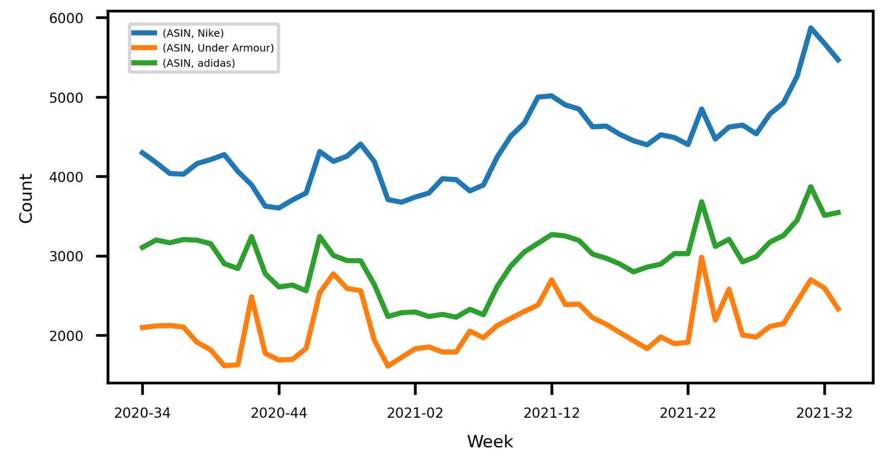
dfAll = dfWideMultiReportsLongExtended
brandsInScope = ["Nike", "adidas", "Under Armour"]

# Create pivot table
dfPivot = pd.pivot_table(dfAll[dfAll['brand'].isin(brandsInScope)],index=["yearWeek"], columns=["brand"], values=["ASIN"], aggfunc='count', fill_value=0)

# Plot data
plt = dfPivot.plot(fontsize=4, figsize=(4, 2))
plt.legend(loc=7, prop={'size': 3}, bbox_to_anchor=(0.23,0.90))
plt.set_ylabel('Count', fontsize=5)
plt.set_xlabel('Week', fontsize=5)
The chart looks like this:
Conclusion
And there you have it. Although we covered quite some ground there is so much more you can do with this data.
I hope we could inspire you with some new ideas to try out.
You can find the full source code of the code above on Github. This of course excludes the search term data as this is only availabe to registered brand owners.
Subscribe to Newsletter
Get the latest Amazon tips and updates delivered to your inbox.
We respect your privacy. Unsubscribe anytime.